Bashford-Adams-Milne integration

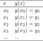
Suppose that you have a table or array of the values of a function

One can perform a linear interpolation\ to obtain $y(x_i+\alpha)$ for
$\alpha<x_{i+1}-x_i$ by assuming that the curve is well approximated by a straight line between adjacent points listed in the table

$y(x_i+\alpha)\approx y(x_i)+{y(x_{i+1}) -y(x_i)\over x_{i+1}-x_i}\, \alpha$

If the points $x_0, x_1, x_2,\cdots$ are evenly spaced with $x_{i+1}-x_i=\delta$ , the Lagrange interpolation can provide better accuracy. Notice that

$y(x+\delta)=y(x)+\delta y'(x)+{1\over 2!} \delta^2 y''(x)+\cdots=e^{\delta {d\over dx}} y(x)=E \, y(x)$

in which $E$ is the shift operator

$E \, y(x)=y(x+\delta)$

Then

(1) $\begin{eqnarray*} y(x+\alpha\delta)&=&y(x)+\alpha\delta \, y'(x)+{1\over 2!} (\alpha\delta)^2 \, y''(x)+\cdots\nonumber\\ &=&e^{\alpha\delta {d\over dx}} y(x)=E^\alpha \, y(x)\end{eqnarray*}$

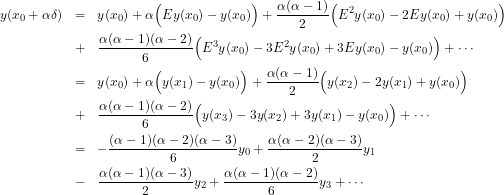
which we can expand as

(2) $\begin{eqnarray*} y(x+\alpha\delta)&=&E^\alpha y(x)=\Big(1+(E-1)\Big)^\alpha y(x)\nonumber\\ &=&y(x)+\alpha(E-1) y(x)+{\alpha(\alpha-1)\over 2!} (E-1)^2 y(x)+{\alpha(\alpha-1)(\alpha-2)\over 3!} (E-1)^3 y(x)+\cdots \end{eqnarray*}$

Collect terms together and use the fact that

$E^n y(x_0)=y(x_0+n\delta)=y(x_n)=y_n$

then

(3) $\begin{eqnarray*}y(x_0+\alpha\delta)&=&y(x_0)+\alpha\Big(Ey(x_0)-y(x_0)\Big)+{\alpha(\alpha-1)\over 2}\Big(E^2y(x_0)-2Ey(x_0)+y(x_0)\Big)\nonumber\\ &+&{\alpha(\alpha-1)(\alpha-2)\over 6}\Big(E^3y(x_0)-3E^2y(x_0)+3Ey(x_0)-y(x_0)\Big)+\cdots\nonumber\\ &=&y(x_0)+\alpha\Big(y(x_1)-y(x_0)\Big)+{\alpha(\alpha-1)\over 2}\Big(y(x_2)-2y(x_1)+y(x_0)\Big)\nonumber\\ &+&{\alpha(\alpha-1)(\alpha-2)\over 6}\Big(y(x_3)-3y(x_2)+3y(x_1)-y(x_0)\Big)+\cdots\nonumber\\ &=& -{(\alpha-1)(\alpha-2)(\alpha-3)\over 6} y_0 +{\alpha(\alpha-2)(\alpha-3)\over 2} y_1 \nonumber\\ &-& {\alpha(\alpha-1)(\alpha-3)\over 2} y_2+{\alpha(\alpha-1)(\alpha-2)\over 6} y_3+\cdots\end{eqnarray*}$

and so on, here correct to third order differences. Notice that if $\alpha=n$ , for $0\le n\le 3$ , we simply obtain $y(x_0+n\delta)=y(x_n)$ . One would use this to get $y(x_0+\alpha\delta)$ for $0<\alpha <1$ in practice, given a set of $y$ -values for regularly-spaced $x$ -values, giving a significant improvement over linear interpolation. It can be used to develop predict-correct numerical integration algorithms (which is why we are interested in it). For example consider a function $y(x)$ and its derivative $y'(x)$ , and apply this to the case $\alpha=-1$ and $y'(x_1)$ instead of $y(x_0)$ , we obtain

$y'(x_0)=4 y'(x_1)-6 y'(x_2) +4 y'(x_3) -y'(x_4)$

Now consider numerically integrating $y'(x)$ from $x_0$ to $x_4=x_0+4\delta$ by Simpson’s rule

$\int_{x_0}^{x_4} y'(x) dx=y(x_4)-y(x_0)={\delta\over 3}\Big( y'(x_0)+4 y'(x_1)+2 y'(x_2)+4 y'(x_3) + y'(x_4)\Big)$

and into this insert the previous interpolation formula to eliminate $y'(x_4)$ on the right side to obtain the interpolation

$y_4=y_0 +{8\delta \over 3}\Big( y'_1 -{1\over 2} y'_2 +y'_3\Big)$

Bashford-Adams-Milne integration is a predict-correct method based on the interpolation formula that we just derived. Consider a differential\equation

$y'=F(y,x)$

and make a guess solution $y_g(x)$ that satisfies the boundary conditions (say $y(0)=0$ ) and build up a table from the guess solution. From the derivatives of the guess solution make the predictions

$y_{n}=y_{n-4} +{8\delta \over 3}\Big( y'_{n-3} -{1\over 2} y'_{n-2} +y'_{n-1}\Big), \quad n\ge 4$

then compute from these new values of the derivatives from

$y'_n =F(y_n, x_n)$

and then correct the prediction using Simpson’s rule

$y_{n}=y_{n-2}+{\delta\over 3}\Big( y'_{n-2}+4 y'_{n-1}+y'_{n}\Big), \quad n\ge 2$

We simply iterate the procedure until desired accuracy is achieved. This method does not suffer from the accumulated errors of Euler. Here is an example in REDUCE for the equation

$y'={dy\over dx}=F(x,y)=1+y^2, \qquad y(0)=0$

on rounded;
operator x,y,yp;
delta:=0.01;
for n:=0:100 do x(n):=n*delta;
% remember y'=!F
!F:=1.0+!Y^2;
y(0):=0.0;
% First guess
for n:=1:100 do y(n):=x(n);
for n:=0:100 do yp(n):=1.0;
% Predictor
% Iterate predict/correct cycle
for m:=0:10 do <<
for n:=4:100 do y(n):=y(n-4)+(8.0*delta/3.0)*(yp(n-3)-0.5*yp(n-2)+yp(n-1));
% Recompute y'
for n:=0:100 do yp(n):=sub(!Y=y(n), !F);
% Correct (note we DON't mess with y(0))
for n:=2:100 do y(n):=y(n-2)+(delta/3.0)*(yp(n-2)+4.0*yp(n-1)+yp(n)) >>;
% compare to exact solution
for n:=0:100 do write y(n), "   ", tan(x(n));

Note that ten cycles gives excellent accuracy ( $y(100 \, \delta)=1.5574072$ versus $\tan(100\, \delta)=1.5574077$ ).

Home 2.0

Bashford-Adams-Milne integration

Related Posts

Bashford-Adams-Milne integration

Published by Jeff on December 26, 2021December 26, 2021

Related Posts

Protected: AI/ML-1. Neural nets in Julia

Algorithms: curve fitting

ML/AI: Feature selection in decision trees (information entropy)