Of all of the interpreted programming languages (python, R, lisp, julia) that I use, R has the best graphics. Here are some examples of an orrery or solar system simulator written in R, with OpenGL graphics.

I wrote it as an R package or library. It contains codes used to find Julian time, eccentric anomalies ψ,F for elliptical and hyperbolic orbits, and the positions of planets in space in terms of ε,Ω,ω,i,a,ψ, and a. These functions are used to draw the orbital trajectory, and to draw a sphere for the object at the position of the Julian date. I also include some tables as Rda data for orbital parameters and times of perihelion passage. For example JDperi.R looks up a planet in the database file and …

#' Julian date conversion
#'
#' Compute Julian calendar time of perihelion in days from database
#' date + time of perihelion passage
#' A utility function, not a user function
#' 
#' @export
#' @param Planet name
#' @return The corresponding Julian time in days for perihelion passage.


JDperi <- function(myplanet){
planetnames <- as.character(planetdb[,1])
if(myplanet %in% planetnames){
which <- grep(myplanet,planetdb$name)
stuff <- strsplit(as.character(planetdb[which,7]),":")
Yr <- as.numeric(stuff[[1]][1])
Mon <-  as.numeric(stuff[[1]][2])
Day <- as.numeric(stuff[[1]][3])
if(Mon <= 2){y <- Yr-1; m <- Mon+12} else {y <- Yr; m <- Mon}
  B <- floor(y/400)-floor(y/100)
 options(digits=10) 
  return(floor(365.25*y)+floor(30.6001*(m+1))+B+1720996.5+Day)}
 else{
 print("No such object in database")
 }
}

Using the library is simple: start R, load it, and run one of the example codes that I include with it. All of these start with the function setup.R which initializes an OpenGL window and coordinate system. I am using the rgl library for OpenGL (https://cran.r-project.org/web/packages/rgl/index.html).

#' Set up the plot window
#'
#' Creates a black field with space-fixe X,Y,Z axes
#' 
#' Imports: rgl
#' 
#' 
#' @export
#' @param MaxL the largest X,Y,Z coordinate value, planes=TRUE to draw XY plane


setup <- function(MaxL, planes=FALSE){
rgl::par3d(windowRect = c(20, 30, 600, 600))
rgl::bg3d("black")
aa <- c(0,0,0)
rgl::plot3d(aa, 
      xlab = "", ylab = "", zlab = "", 
      type = "p", col = "red", 
      xlim = c(-MaxL,MaxL), ylim = c(-MaxL,MaxL), zlim = c(-MaxL,MaxL), 
      aspect = c(3,3,3), 
      size = 0,
      main = "", sub = "", ann = FALSE, axes = FALSE)
# draw the space-fixed coordinate axes
rgl::arrow3d(c(0,0,0),c(MaxL,0,0), type = "lines", s=1/10,  col = "green")
rgl::text3d(MaxL+0.1,0,0.1,"X",cex=0.9,col = "green")
rgl::arrow3d(c(0,0,0),c(0,MaxL,0), type = "lines",  s=1/10, col = "green")
rgl::text3d(0,MaxL+0.1,0.1,"Y",cex=0.9,col = "green")
rgl::arrow3d(c(0,0,0),c(0,0,MaxL), type = "lines",  s=1/10, col = "green")
rgl::text3d(0,0,MaxL+0.1,"Z",cex=0.9,col = "green")
if (planes==TRUE){rgl::planes3d(0,0,1, col="white",alpha=0.3)}
# The sun
rgl::spheres3d(0,0,0,col="yellow",radius=0.2*MaxL)
}

So here are some examples: let’s plot a transfer orbit that takes us from Earth to mars in 240 days, I use the Lambert transfer solver that I included in the library.

library(Orerrey)
setup(2)
plot2Dorbit("Earth")
plot2Dorbit("Mars")
locate2D("Earth",JD(2020,10,10,0,0,0),"blue",0.15)
locate2D("Mars",JD(2020,10,10,0,0,0),"red",0.15)
locate2D("Mars",JD(2021,6,10,0,0,0),"red",0.15)
# 243 days
out <- Lambert(0.9986850602,0.2874308514,1.660891063, 2.479240937)
# -1 0
plot_transfer(0.2874308514,out,10)
now <- JD(2020,10,10,0,0,0)
for (days in seq(0,240,10)){
locate2D("Earth",now+days,"blue",0.15)
locate2D("Mars",now+days,"red",0.15)
locate_transfer(0.2874308514,out,10,days)}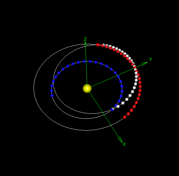

You can use the mouse to zoom, rotate, or reposition the plot in the rgl window, of course these png’s cannot be manipulated this way…

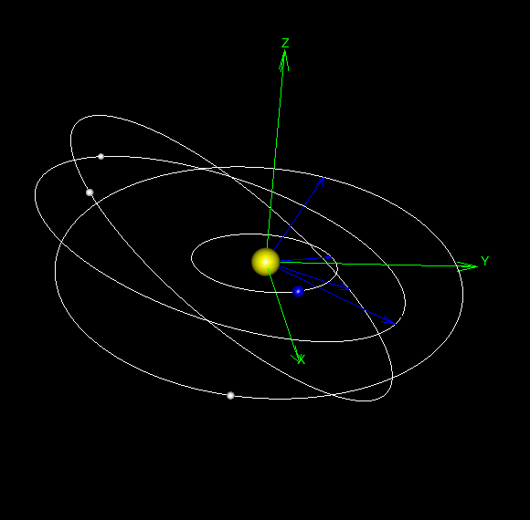
As another example let’s look at the asteroid orbits for Ceres, Pallas and Juno. The blue arrows point to perihelia, the blue ball is the Earth.

# Earth and 'roids
setup(3)
planetdb[,1]
for(name in as.character(planetdb[c(4,10,13,14),1])){
plot_orbit(name)}
locate("Earth",JD(2020,10,11,12,0,0),"blue",0.25)
roids <-c("Ceres","Juno","Pallas")
for(name in roids){
locate(name,JD(2020,10,11,12,0,0),"white",0.15)}

Finally let’s look at the trajectory of Oumuamua, and see just how close it came to the Earth as it passed through the solar system.

# Closest approach to Earf
library(Orerrey)
setup(1.25)
JD(2017,10,15,0,0,0)
# 2458041.5
plot_orbit("Earth")
locate("Earth",JD(2017,10,15,0,0,0),"blue",0.2)
Trajectory(3,1.2723, 1.20113,0.428827,4.22038,21.4221)
locate_extra_solar(2458041,2458006,1.2723, 1.20113,0.428827,4.22038,21.4221,0.125,"white")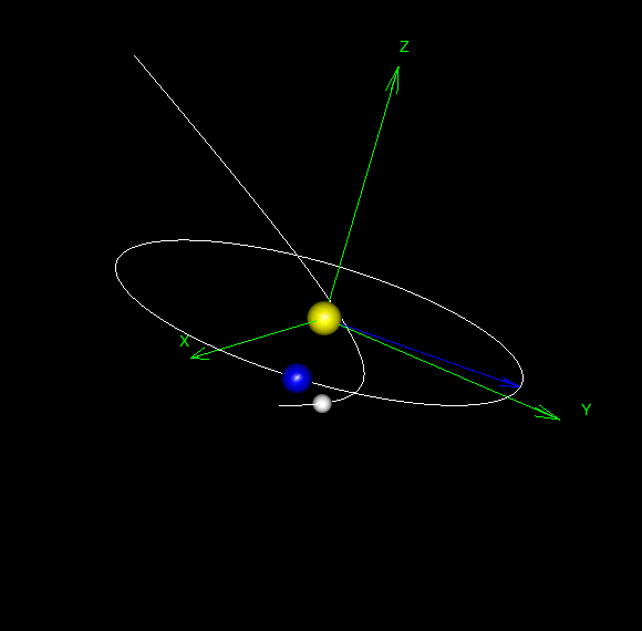

Rotate the figure a bit…

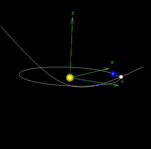
It almost looks like it was aimed at us.