Quantum spin-chains-III. Density Matrix Renormalization Group

The most powerful ideas that we will study in Physics 715 are related to the scaling hypothesis, which provides the renormalization group methods (real space, momentum space, and DMRG). These methods allow us to study the physics of very large interacting systems in one energy or scale regime, as an effective “field” theory.
The density matrix renormalization group (DMRG) is a numerical variational technique devised to obtain the low-energy physics of quantum many-body systems with high accuracy. It is currently a dominant computational tool in condensed matter physics.
“Its main advantages are the ability to treat unusually large systems at high precision at or very close to zero temperature …”, so we will use it to establish the numerical value of the ground state energy in the quantum spin- $1/2$ Heisenberg chain that we have examined in two previous posts.
All renormalization group methods involve a step called decimation, in which a number of degrees of freedom are averaged over in order to create an effective Hamiltonian system for the remaining part of the system.

There are two versions, let’s look at the “infinite system version”, which consists of a series of steps that are cycled through.

$\bullet$ In the initialization stage two blocks $S,E$ of the system, both of size $\ell$ (meaning $\ell$ sites) both of which are small enough to be exactly solved, are introduced. The basis states of each block form a tensor space of size $d^\ell$ , $d=2$ for spin- $1/2$ spanned by $|S\rangle=\{|s_1\rangle\otimes |s_2\rangle\otimes\cdots\otimes|s_\ell\rangle\}$ and similarly for $|E\rangle$ .

$\bullet$ A spin is added to each block, creating systems $S\bullet$ and $\bullet E$ with bases $\{|S\rangle\otimes|s\rangle\}$ and $\{|s'\rangle\otimes |E\rangle\}$ respectively.

$\bullet$ A superblock $S\bullet\bullet E$ of size $2\ell+2$ is formed, with Hamiltonian
$H_{S\bullet\bullet E}$ . The ground state $|\psi\rangle$ of this Hamiltonian is found by sparse-matrix methods.
$\bullet$ If we iterate this process, replacing each block with the superblock and repeating the process, the size of the basis of the superblock Hamiltonian grows exponentially.
The idea of RG methods is to decimate or reduce the size of the basis judiciously after each iteration so that the basis does not grow at all, even as the chain increases in length with each iteration. In DMRG this is done as follows. Note that the ground state $|\psi\rangle$ of the superblock is writable as entangled tensor products of “S” and “E” vectors

$|\psi\rangle=\sum_{|s'\rangle\in S\bullet}\sum_{|e'\in \bullet E}\psi_{s',e'}|s'\rangle\otimes|e'\rangle$

$\bullet$ Construct the density matrix $\rho=|\psi\rangle\langle\psi|$ (a $d^{\ell+1}\times d^{\ell+1}$ matrix) from the ground state. Construct the reduced density matrix $\rho_{S\bullet}$ by tracing out the states of $\bullet E$

$\rho_{S\bullet}=Tr_{\bullet E}|\psi\rangle\langle\psi|=\sum_{|s'\rangle\in S\bullet}\sum_{|s"\rangle\in S\bullet} \rho_{s',s"}|s'\rangle\langle s"|$

$\bullet$ Find the basis $|i\rangle$ of $S\bullet$ in which this is diagonal

$\rho_{S\bullet}=\sum_i w_i|i\rangle\langle i|$

In julia this is simple: use the built-in eigensolver to find he eigenvalues $w$ (a diagonal matrix) and eigenvectors $V$ of $\rho_{S\bullet}$ .

Keep in mind that the size of the basis of $S\bullet$ is $d^{\ell+1}$ and of $S$ the basis $|S\rangle$ has size $d^\ell$ . Select $d^\ell$ of the $|i\rangle$ vectors with the largest weights $w_i$ , (in julia just keep the last $d^\ell$ columns of $V$ corresponding to the $d^\ell$ largest eigenvalues $w$ because eigvals/eigvecs sorts from smallest to largest) and call it the matrix $T$ , which is $d^{\ell+1}\times d^\ell$ , consisting of the $d^\ell$ column vectors of the largest weight $|i\rangle's$ . If $w_1<w_2<w_3\cdots$ then $T=[|1\rangle,|2\rangle, \cdots, |d^\ell\rangle]$ .

You will eventually see that this represents the states maximally entangled with the ground state.
$\bullet$ The Hamiltonian $H_{S\bullet}$ for $S\bullet$ is $d^{\ell+1}\times d^{\ell+1}$ . Create a new Hamiltonian $H_{S'}=T^\dagger\cdot H_{S\bullet}\cdot T$ which is $d^\ell\times d^\ell$ , the same size as $H_S$ . This becomes the block Hamiltonian for the next step.

$\bullet$ You need to transform the spin operators for the end-spins too, $\bm{s}_{S',end}=T^\dagger\cdot \bm{s}_{S\bullet,end}\cdot T$ in order to build the Hamiltonian for the next iteration from these new blocks

$H_{superblock,new}=H_{S'}+J\bm{s}_{S',end}\cdot\bm{s}+J\bm{s}\cdot\bm{s}'+J\bm{s}'\cdot \bm{s}_{end,E'}+H_{E'}$

and repeat the process of finding the (new) ground state $|\psi\rangle$ .

We will try to use initial “S,E” systems consisting of single spins, so a superblock will have four spins and each iteration will “add” two. This is naive since it underestimates how many states are well-entangled with the ground state in long chains. The larger the state-chains are, the better. But we still get very encouraging results.
So start out with each block (both $S,E$ ) having {\bf one} spin, so that initially $H_S=0$ and $H_E=0$ (both are $2\times 2$ zero matrices). The superblock Hamiltonian is then (tensor products are associative)

$H_{superblock}=J\Big(P\otimes I\otimes I+I\otimes P\otimes I+I\times I\otimes P\Big), \quad I=\left(\begin{array}{cc} 1&0\\ 0&1\end{array}\right)$

The reduced density matrix $\rho_{S\bullet}=Tr_{\bullet E}|\psi\rangle\langle\psi|$ is then a $4\times 4$ in the basis for the spin $s_1$ of $S$ and the extra spin $s_2$ . The $T$ matrix made from the two largest weight eignvalues of $\rho_{S\bullet}$ is $4\times 2$ . We have explicitly then (with $\bm{s_2}=(s_x,s_y,s_z)$ )

$H_{S'}=T^\dagger\cdot(H_{S}\otimes I+P)\cdot T, \quad \bm{s}_{S',end}=T^\dagger\cdot(I\otimes \bm{s})\cdot T$

$\bm{s}_{end,E'}=T^\dagger\cdot(\bm{s}\otimes I)\cdot T, \quad H_{E'}=T^\dagger\cdot(I\otimes H_{E}+P)\cdot T$

all of which are $2\times 2$ matrices.
The code in julia is below, with lots of documentation strings, you should try to rewrite it so that the start-sytems can be two or three spin chains.

using LinearAlgebra,Kronecker,DataFrames, Gaston

DMRG=function(num)
gs=zeros(num)
sx=[0 1.0;1 0]/2.0;sy=[0 -im;im 0]/2.0;sz=[1.0 0;0 -1]/2.0;
u2=[1.0 0;0 1.0]; u4=u2⊗u2;
# note u2[:,1] and u2[:,2] form a spin basis for single site
#  u4[:,1], ..., u4[:,4] form a spin basis pair of sites
# System spin operators for spin 1,2
Ssx0=[sx⊗u2,u2⊗sx];Ssy0=[sy⊗u2,u2⊗sy];Ssz0=[sz⊗u2,u2⊗sz];
Ssx=Ssx0;Ssy=Ssy0;Ssz=Ssz0;
# Env spin operators for spin 1,2
Esx0=[sx⊗u2,u2⊗sx];Esy0=[sy⊗u2,u2⊗sy];Esz0=[sz⊗u2,u2⊗sz];
Esx=Esx0;Esy=Esy0;Esz=Esz0;
# initial Hamiltonians
HS=zeros(4,4); HE=zeros(4,4);
HSp=HS+Ssx0[1]*Ssx0[2]+Ssy0[1]*Ssy0[2]+Ssz0[1]*Ssz0[2];
HEp=HE+Esx0[1]*Esx0[2]+Esy0[1]*Esy0[2]+Esz0[1]*Esz0[2];
# Superblock Hamiltonian
H=HSp⊗u4+u4⊗HEp+Ssx0[2]⊗Esx0[1]+Ssy0[2]⊗Esy0[1]+Ssz0[2]⊗Esz0[1];
for cycles in 1:num
# get most negative, the first, they are sorted
psi0=eigvecs(H)[:,1]
gs[cycles]=eigvals(H)[1]/(2.0*(cycles-1.0)+4.0);
# Create reduced |psi0><psi0| for S, E and the transformation matrices
# get largest two eigvalue vectors
rhoS=sum(((u4⊗u4[:,j]')*psi0)⊗((u4⊗u4[:,j]')*psi0)' for j in 1:4);
TS=eigvecs(rhoS)[:,3:4]
rhoE=sum(((u4[:,j]'⊗u4)*psi0)⊗((u4[:,j]'⊗u4)*psi0)' for j in 1:4);
TE=eigvecs(rhoE)[:,3:4]
# the trans matrices are made from eivs corresp to two
# largest eigs of the rhoS, rhoE 

#Transform operators
HS=(TS'*HSp*TS)⊗u2;
Ssz[1]=(TS'*Ssz0[2]*TS)⊗u2;
Ssy[1]=(TS'*Ssy0[2]*TS)⊗u2;
Ssx[1]=(TS'*Ssx0[2]*TS)⊗u2;
HE=u2⊗(TE'*HEp*TE);
Esz[2]=u2⊗(TE'*Esz0[1]*TE);
Esy[2]=u2⊗(TE'*Esy0[1]*TE);
Esx[2]=u2⊗(TE'*Esx0[1]*TE);
# New superblock Hamiltonian
HSp=HS+Ssx[1]*Ssx[2]+Ssy[1]*Ssy[2]+Ssz[1]*Ssz[2];
HEp=HE+Esx[1]*Esx[2]+Esy[1]*Esy[2]+Esz[1]*Esz[2];
H=HSp⊗u4+u4⊗HEp+Ssx[2]⊗Esx[1]+Ssy[2]⊗Esy[1]+Ssz[2]⊗Esz[1];
H=(H+H')/2.0;
end
iters=[j for j in 0:num-1]
dat=DataFrame(L=vec(iters),E=vec(gs));
print(gs[num-1]);
print("\n")
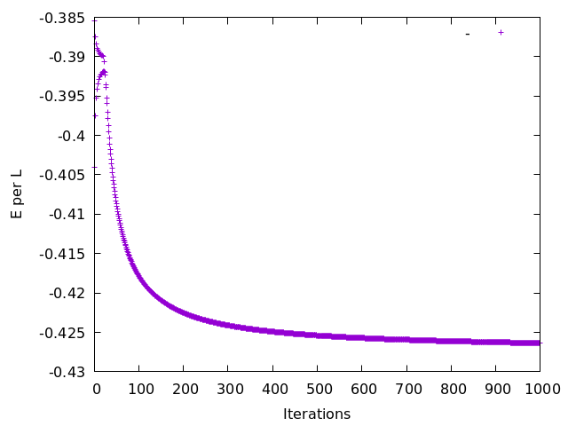
plot(dat.L,dat.E, Axes(xlabel =:Iterations, ylabel=:E_per_L),legend=:- )
end

With an initial system size of one spin, it converges on the true ground state energy per spin of $-0.4401$ (computed by Bethe ansatz) rather slowly, after $3000$ cycles reaching $-0.43700$ . Increasing the initial system size to two spins lets $E_0/L$ reach $-0.439878$ within $150$ cycles. What is being computed here is the infinite-chain ground state energy per spin. Email me for a download link for the code.