Our hand-made FFT code from FFT-II is very fast (order for a full Fourier transform of a length – input), but we made no optimizations. The julia FFTW library (which uses routines from the C FFTW library) is highly optimized and very fast. I wrote our code in the previous post to emulate its input and output as closely as possible so that comparison is easy.

using FFTW
using Plots
N=256
L=5
t = range(-L, stop=L, length=N)
# -5.0:0.0392156862745098:5.0
# note 10/255=0.0392156862745098
k=1:256
shiftedks = fftshift(fftfreq(N)*N)
# -128:1:127

# our input
signal = cos(2*π*3 .* t)
FFTsignal = fftshift(fft(signal))

plot(x, f, title = "signal(t)", xlabel = "Time", ylabel = "f(t)")

plot((1/(2*L))*shiftedks, abs.(FFTsignal), title = "FFT", xlabel = "ω/2π", ylabel = "F(ω)")

The function fftshift(fftfreq(N)*N) creates a set of symmetric (about ) frequencies, which we did by hand, based on the size of the sample which again must be a power of . We do some rescaling of the shifted k’s when we make the plots of the FFT’ed signal, which again is two nice delta functions.
Reading/parsing FITS files
Many of you will need to analyze spectra stored in FITS file formats. You can get a nice FITS file viewer “fv” that reads headers and prints out datafields, or you can use the FITSIO julia library to read out useful things in the header.
I downloaded a spectrum from the NSO historical library https://nispdata.nso.edu/ftp/FTS_cdrom/ and read its header to get the start/stop wavenumbers, and the wavenumber spacing (DELW). I also read the data axis into an array “I” (intensities) and create an array “k” so that I can print out pairs

using FITSIO, VegaLite, DataFrames
f = FITS("881115R0.005")
# one HDU
header = read_header(f[1])
# stop/start wavenumbers
wstart=header["WSTART"]
wstop=header["WSTOP"]
# spacing
delw=header["DELW"]
# (wstop - wstart) / delw = NPO 
npo=header["NPO"]
# read length of the data axis of HDU
naxis1=header["NAXIS1"]
I=read(f[1])
k=[wstart+j*delw for j in 1:npo]
# 602112-element Vector{Float32}
close(f)

Some software that processes these very large spectra (this file had 602112 lines) expects the data to be stored in a binary format, which is about 20% the size of an ASCII data file, so we can print our pairs or just the values to a binary file (as binary Float32 data)

""" Write FITS file intensities to binary file"""
binwrite=function(Intensities,outfile)
  open(outfile, "w") do file
         for j in 1:length(Intensities)
         write(file, Float32.(Intensities[j])) # write a Float64
         end
  end

Once we have the pairs, we can do things like find centers of gravities of lines, search for strong/high lines, and make plots of parts of the spectrum. I find that the VegaLite plotting library works best for this

"""COG(L,R,k,I)=Center of gravity of intensities for L<= indices <=R
   k is set of wavenumbers, I is FITS intensities"""
COG=function(L,R,k,I)
sum(k[L:R,1] .* I[L:R,1])/sum(I[L:R,1])
end

"""absCOG(L,R,k,I)=Center of gravity of abs(intensities) for L<= indices <=R
   k is set of wavenumbers, I is FITS intensities"""
absCOG=function(L,R,k,I)
sum(k[L:R,1] .* abs.(I[L:R,1]))/sum(abs.(I[L:R,1]))
end

"""Display(L,R,k,I) plots intensities for L<= indices <=R
   k is set of wavenumbers, I is FITS intensities"""
Display=function(L,R,k,I)
dat=DataFrame(k=vec(k[L:R]),I=vec(I[L:R]))
dat |> @vlplot(width=1000, :line, :k, :I)
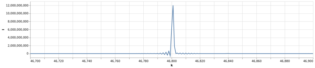
end

For example from this datafile let’s load VegaLite and plot the region around one of the high-intensity lines using my Display function for and :