The gnu plotutils library gives you a useful filter program called ode that accepts commands in a simple language for numerically integrating equations of motion using fourth order adaptive step-size Runge-Kutta integration. It is as fast and accurate as can be, and is very simple to use.
Read the docs (install with “sudo apt install plotutils”). Write your commands into a text file, for example for solving the Foucault pendulum motion as illustrated in Physics 311 and 711…

g=9.8
L=3
w=0.2
x'=p
y'=q
p'=-(g/L)*x+2*w*q
q'=-(g/L)*y-2*w*p
p=0
q=0
x=1
y=1
print x,y
step 0,10

Save this as “Foucault.ode”, and in a shell, assuming that you are running Xwindows, cat the script into ode and pipe its output into the graph command, also provided by plotutils

cat Foucault.ode | ode |graph -T X

and out comes your plot, almost instantaneous

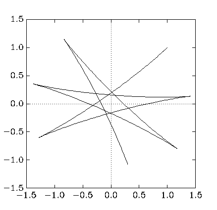
The julia DifferentialEquations library (https://diffeq.sciml.ai/stable/tutorials/ode_example/) works in a nearly identical fashion…

using DifferentialEquations, Plots

# parmeters (the p's)
g=9.8
L=3.0
w=0.2

function Foucault!(du,u,p,t)
du[1]=u[3]
du[2]=u[4]
du[3]=-(g/L)*u[1]+2.0*w*u[4]
du[4]=-(g/L)*u[2]-2.0*w*u[3]
end

x₀=1;y₀=1;vx₀=0; vy₀=0
tspan = (0.0,10.0)  
u₀=[x₀,y₀,vx₀,vy₀]
prob = ODEProblem(Foucault!,u₀,tspan)
sol = solve(prob)
plot(sol,vars=(1,2))

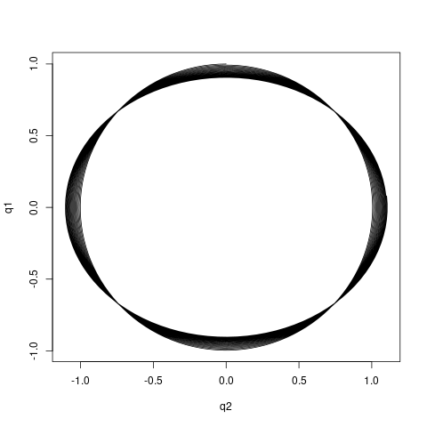
In R we have the DESolve package, and all three of these code packages are so similar that if you know one you know them all. Here we solve an oscillator EOM in which the force constant increases slowly with time. What is cool is the the phase space plot of versus shows the adiabatic invariance of the action , the area within the phase space orbital curve is constant.

# in R
library(deSolve)
osc <- function(t,q,pars){
   with(as.list(c(q,pars)),{
   q1_dot <- q2
   q2_dot <- -(1+eps*t)*q1
   return(list(c(q1_dot,q2_dot)))})
}
pars <- c(eps=0.005)
qini <- c(q1=1,q2=0)
times <- seq(0,100,by=0.05)
soln <- ode(qini,times,osc,pars)
plot(q1~q2,data=soln,type = "l", lwd = 1)

png(file="AdiaInv.png")
plot(q1~q2,data=soln,type = "l", lwd = 1)
dev.off()