ML/AI: Probability and statistics-VI. Prediction and information entropy

Let $Y$ be a random variable and $E[Y]$ is expectation. Note that $E[(Y-c)^2]$ is minimal when $c=E[Y]$

$E[(Y-c)^2]=E[Y^2]-2cE[Y]+c^2, \qquad {\partial\over \partial c}E[(Y-c)^2]=0=2(c-E[Y])$

and section 7.6 of Ross “A First Course in Probability” proves the important theorem

$E[(Y-g(X))^2]\ge E[(Y-E[Y|X])^2]$

so that the left side is minimal when $Y=E[Y|X]$ , implying that we can use the theorem to predict an outcome of $Y$ subject an outcome of $X$ having occured, then the best guess for the outcome of $Y$ is $g(X)=E[Y|X]$ .
A nice example is afforded by problem 7.33; predict the number of rolls of a fair die necessary to roll a $6$ if on the first roll you got a $5$ , you will find that it is $7$ . This is because we are dealing with a geometric random variable, the probability of success on independent trial $n$ with failures for trials $<n$ is

$\wp(X=n)=(1-p)^{n-1}p$

so the expected $n$ is $E[X]=\sum_{n=1}^\infty np(1-p)^{n-1}={1\over p}$ , so if on the first roll we get a $5$ , we have to roll $n=1/(1/6)=6$ more times before we expect to get a $6$ .

What is the best linear estimate of the next or expected $Y$ ? Extremize

$Z=E[(Y-(a+bX))^2]$

$=E[Y^2]-2a E[Y]-2b E[XY]+a^2+2ab E[X]+b^2 E[X^2]$

with respect to $a$ and $b$ , which results in

${\partial Z\over \partial a}=0=2\Big(a+b E[X]-E[Y]\Big)$

${\partial Z\over \partial b}=0=2\Big(a E[X]+b E[X^2]-E[XY]\Big)$

$a={E[Y] E[X^2]-E[X]E[XY]\over E[X^2]-E^2[X]},\quad b={E[XY]-E[X]E[Y]\over E[X^2]-E^2[X]}$

which you may recall from teaching Physics 103, 201 or 207 lab are exactly the least-squares fit formulas for the best straight line fitting a collection of data. Therefore the best (linear) predictor of $Y$ with respect to $X$ is $a+bY=\mu_y+{\rho \sigma_y\over \sigma_x}(X-\mu_x)$ .

Example. German tank problem During WW-II (the Great Patriotic War) the Allies tried to estimate the number of German tanks from the knowledge that each had a unique serial number, which were sequential integers $1,2,\cdots, N$ . From a sample size of $k$ captured/destroyed tanks and the largest serial number $m$ in the sample they tried to estimate $N$ , the largest serial number. They were able to do so quite accurately. We will need only the identity

$\sum_{m=k}^N {m\choose k}={N+1\choose k+1}$

which we prove by induction, it is true if $k=N$ ,

$\sum_{m=k}^{N+1} {m\choose k}=\sum_{m=k}^{N} {m\choose k}+{N+1\choose k}={N+1\choose k+1}+{N+1\choose k}={N+2\choose k+1}$

Tanks are numbered $1,2,\cdots, N$ . Sample $k$ , the largest serial number in sample is $m$ , estimate $N=\hat{N}(m,k)$ . Ansatz

$\hat{N}=m+g(m,k)\equiv m(1+b/k), \quad \mbox{some}\quad b$

so conjecture that

$\hat{N}= m(1+1/k)-1$

Let $X$ be the random variable for the observed largest serial number observed, $m$ is the observed value. If we have a sample of size $k$ , the smallest that the observed $m$ can be is $k$ (sample could have all of the lowest serial numbers $1,2,\cdots, k$ ), so that the range of $m$ is $k\le m\le N$ . We find that

$\wp(X=m)={{m\choose k}-{m-1\choose k}\over {N\choose k}}={{m-1\choose k-1}\over {N\choose k}}$

Proof: If the largest is $m$ , then we must choose $k-1$ other tanks n the sample from the $m-1$ serial numbers lower than $m$ , so $\wp(X=m)={{m-1\choose k-1}\over {N\choose k}}$ .
The expected value of $X$ is

$E[X]=\sum_{m=k}^N m{{m-1\choose k-1}\over {N\choose k}}=\sum_{m=k}^N m{(m-1)!\over (k-1)!(m-k)!}{k!(N-k)!\over N!}$

$={kk!(N-k)!\over N!}\sum_{m=k}^N{m\choose k}={kk!(N-k)!\over N!}{N+1\choose k+1}={k(N+1)\over k+1}$

Then

$N=E[X](1+1/k)-1$

I would like to thank E. Basso for introducing this problem to me.

Unpredictability (the entropy or surprise)
The concept of “surprise” measures how surprised we would be if event $E$ occurred, and so is a measure of unpredicatbility. We have several axioms in its formulation
$\bullet$ $S(1)=0$ , we are not surprised that a sure thing occurs. Sure things are highly predictable.
$\bullet$ $S(p)$ strictly decreases with $p=\wp(E)$ , we are more surprised when unlikely events occur.
$\bullet$ $S(p)$ is a continuous function of $p$ , so small $p$ -changes result in small $S$ -changes.
$\bullet$ $S(pq)=S(p)+S(q)$ , since if $p=\wp(E)$ and $q=\wp(F)$ and $E,F$ are independent events, then $\wp(EF)=pq$ . $S(pq)-S(p)$ is the additional surprise from the knowledge that if told $E$ has occurred, then told $F$ has occurred.
$\bullet$ The form that satisfies all axioms is

$S(p)=-C\log_2(p)$

Let $X$ have possible values $x_1,x_2,\cdots, x_n$ with probabilities $p_1,p_2,\dots, p_n$ .
\item The expected surprise upon learning the value of $X$ is

$H(X)=-\sum_{i=1}^n p_i\ln p_i$

which is the information entropy of $X$ .

Example
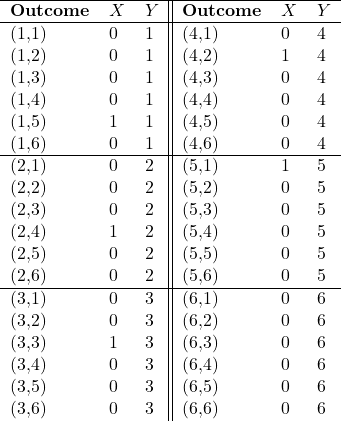
A pair of fair dice are rolled. Let $X=\left\{\begin{array}{ll} 1 & \mbox{sum of dice is 6}\\ 0 &\mbox{otherwise}\end{array}\right.$ . Let $Y$ be the value of the first dice. Compute $H(Y), H_Y(X), H(X,Y)$ .

$\wp\{X=0\}={31\over 36}, \qquad \wp\{X=1\}={5\over 36}$

$H(X)=-{31\over 36}\log_2\Big({31\over 36}\Big)-{5\over 36}\log_2\Big({5\over 36}\Big)=0.581321498764$

$\wp\{Y=i\}={1\over 6}, \qquad i=1,2,3,4,5,6$

$\qquad H(Y)=-6\cdot{1\over 6}\cdot\log_{2}\Big({1\over 6}\Big)=2.58496250072$

$\wp\{X=0|Y=i\}=\left\{\begin{array}{ll} {5\over 6} & i=1,2,3,4,5\\ 1 & i=6\end{array}\right.$

$\wp\{X=1|Y=i\}=\left\{\begin{array}{ll} {1\over 6} & i=1,2,3,4,5\\ 0 & i=6\end{array}\right.$

$H_{Y=1,2,3,4,5}(X)=-{5\over 6}\log_2\Big({5\over 6}\Big)-{1\over 6}\log_2\Big({1\over 6}\Big)=0.650022421648$

$H_{Y=6}(X)=0$

$H_Y(X)=5\cdot\Big(0.650022421648\Big)\Big({1\over 6}\Big)+\Big(0\Big)\Big({1\over 6}\Big)=0.541685351374$

Example
A coin with probability $p=2/3$ of coming up heads is flipped $6$ times. Compute the entropy of the experiment.

Convert to $\log_{2}$ by dividing by $\ln 2$ and sum the last column

$H=-\sum_i p_i \log_2 p_i=2.23007$

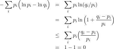
A lemma of great importance in statistical mechanics:
let $\sum_i p_i=1$ and $\sum_i q_i=1$ , then

$-\sum_i p_i \, \ln p_i\le -\sum_i p_i \, \ln q_i$

with equality occurring when each $q_i=p_i$ . This uses $\ln(1+x)\le x$ for $x>-1$ only and was used by Gibbs to prove maximality of the Boltzmann entropy.

(1) $\begin{eqnarray*}-\sum_i p_i \Big(\ln p_i-\ln q_i\Big)&=&\sum_i p_i \ln(q_i/p_i)\nonumber\\ &=&\sum_i p_i \ln\Big(1+{q_i-p_i\over p_i}\Big)\nonumber\\ &\le & \sum_i p_i \Big({q_i-p_i\over p_i}\Big)\nonumber\\ &=&1-1=0\nonumber\end{eqnarray*}$

Uncertainty in a random variable (on average) decreases when a second random variable is measured. This makes intuitive sense (the second measurement reveals information about the first). Since entropy is a measure of the average surprise that you experience when $X$ is measured, $H(X)$ is a measure of the uncertainty in the value of $X$ . In other words

$H_Y(X)\le H(X)$

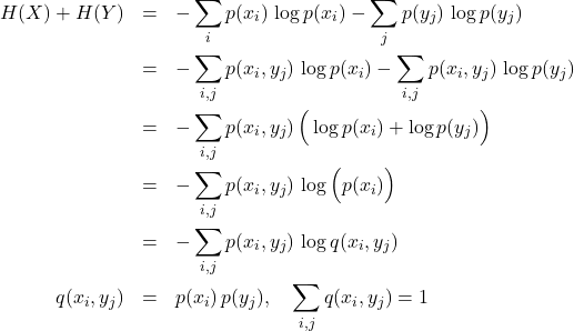
We expand on the proof in Ross’s Chapter 9. Consider two sets of discrete variables $x,y$ :

$p(x_i)=\sum_j p(x_i, y_j), \qquad \sum_{i,j} p(x_i, y_j)=1$

$\Big(\sum_i p(x_i)\Big)\Big(\sum_j p(y_j)\Big)=1\cdot 1=1$

then

(2) $\begin{eqnarray*}H(X)+H(Y)&=& -\sum_i p(x_i) \, \log p(x_i)-\sum_j p(y_j) \, \log p(y_j)\nonumber\\ &=& -\sum_{i,j} p(x_i, y_j) \, \log p(x_i)-\sum_{i,j} p(x_i, y_j) \, \log p(y_j)\nonumber\\ &=& -\sum_{i,j} p(x_i, y_j) \, \Big(\log p(x_i)+\log p(y_j)\Big)\nonumber\\ &=& -\sum_{i,j} p(x_i, y_j) \, \log \Big(p(x_i)\Big)\nonumber\\ &=& -\sum_{i,j} p(x_i, y_j) \, \log q(x_i,y_j)\nonumber\\ q(x_i, y_j)&=& p(x_i) \, p(y_j), \quad \sum_{i,j}q(x_i, y_j)=1\end{eqnarray*}$

Lemma:

$-\sum_{i,j} p(x_i, y_j) \, \log q(x_i, y_j)\geq -\sum_{i,j} p(x_i, y_j) \, \log p(x_i, y_j)=H(X,Y)$

so we have

$H(X)+H(Y)\ge H(X,Y)$

with equality when $X$ , $Y$ are independent. But we also have

$H(X,Y)=H(Y)+H_Y(X)\quad\implies\quad H_Y(X)\le H(X)$

For a variable with two outcomes with probabilities $p$ and $1-p$

$H=-p\log_2 p-(1-p)\log_2(1-p)$

is maximal when $p=1/2$ , which certainly erases any chances that you have of predicting the outcome, both outcomes are equally likely. $H=1$ for $p=1/2$ , and is zero by construction if $p=0,1$ since one or the other outcome is a sure thing. Gini impurity has the same properties

$G=\sum_k \wp(k)(1-\wp(k))$

For our two outcome case $G=2p(1-p)$ is maximal again at $p=1/2$ and zero for sure bets $p=0,1$ . Entropy and Gini impurity are both used for feature selection in the construction of tree classifiers.

Home 2.0

ML/AI: Probability and statistics-VI. Prediction and information entropy

Related Posts

ML/AI: Probability and statistics-VI. Prediction and information entropy

Published by Jeff on November 27, 2021November 27, 2021

Related Posts

Protected: AI/ML-1. Neural nets in Julia

Protected: AI/ML-2. Flux.jl crash course. Layers, models, autodiff.

Algorithms: SVD (singular value decomposition)