Let ![]() be a random variable with the property that there exists a non-negative function
be a random variable with the property that there exists a non-negative function ![]() defined on
defined on ![]() such that
such that
![]()
then ![]() is a continuous random variable and
is a continuous random variable and ![]() is its probability distribution function or PDF (
is its probability distribution function or PDF (![]() ). An example is
). An example is ![]() is the probability that a quantum
is the probability that a quantum ![]() measurement returns a value between
measurement returns a value between ![]() and
and ![]() .
.
We have some simple properties
![]()
and
![]()
The cumulant is a very useful construction
The cumulant is a very useful construction
![]()
Uniform random variable
![]()
Microcanonical distribution
In statistical mechanics the microcanonical distribution applies to a system of constant energy and assumes that all states, which are specification of coordinate ![]() and conjugate momentum
and conjugate momentum ![]() for which
for which ![]() are equally likely, so
are equally likely, so ![]() . For a harmonic oscillator
. For a harmonic oscillator ![]() and the number of states of energy between
and the number of states of energy between ![]() and
and ![]() is
is
![]()
Restrict attention to ![]() and
and ![]() , then for fixed
, then for fixed ![]() there is only a single independent degree of freedom, either
there is only a single independent degree of freedom, either ![]() or
or ![]() , which is not uniformly distributed. Using
, which is not uniformly distributed. Using
![]()
![]()
the number of states accessible per unit energy is
![]()
![]()
![]()
![]()
For the full phase space we have ![]() which increases with energy (what we call a normal system).
which increases with energy (what we call a normal system).
If we sample the ![]() -state of an oscillator we are most likely to get a
-state of an oscillator we are most likely to get a ![]() value that the oscillator spends most of its time in,
value that the oscillator spends most of its time in, ![]()
![]()
![]()
Normal random variable
![]()
One of its most important properties is that if ![]() is normally distributed with parameters
is normally distributed with parameters ![]() , then
, then ![]() is normally distributed with parameters
is normally distributed with parameters ![]() . This illustrates the use of the cumulant
. This illustrates the use of the cumulant
![]()
![]()
![]()
Exponential and Gamma distributions
The exponential distribution has a parameter ![]() , and pdf and cumulant
, and pdf and cumulant
![]()
![]()
The exponential distribution is memoryless, if ![]() represents a “waiting time”, until an event occurs, there is no dependence on how much time has already elapsed (i.e.
represents a “waiting time”, until an event occurs, there is no dependence on how much time has already elapsed (i.e. ![]() ). The only continuous memory-less distributions are exponential.
). The only continuous memory-less distributions are exponential.
The Gamma distribution also has parameters ![]() ,
,
![Rendered by QuickLaTeX.com \[f(x)=\left\{\begin{array}{ll} {\lambda\over \Gamma(t)} (\lambda x)^{t-1}\, e^{-\lambda x} & x\ge 0\\ 0 & x<0\end{array}\right.\]](http://abadonna.physics.wisc.edu/wp-content/ql-cache/quicklatex.com-d70a2116b820c333e3881b2512746d5d_l3.png)
An example is the canonical distribution for a normal system of ![]() particles, one whose entropy increases with energy as a power of the energy
particles, one whose entropy increases with energy as a power of the energy
![]()
![]() ,
, ![]()
Normal random variable cumulant
Begin with the pdf (probability distribution)
![]()
for which (let ![]() ,
, ![]() )
)
![]()
![]()
![]() is called the error function
is called the error function
![]()
![]()
Note that
![]()
The relation between the two is
![]()
![]()
The error function is included in the function libraries of most CAS systems such as REDUCE, Maple and Mathematica.
Example
![]() is normally distributed with
is normally distributed with ![]() . Compute
. Compute ![]() . We will get
. We will get ![]() .
.
% In REDUCE...
on rounded;
load_package specfn;
% Check table on Ross p. 131
0.5*(1+erf(3.4/sqrt(2)));
%example 3a in Chapter 5 of Ross
0.5*(1+erf((5-3)/(3*sqrt(2))))-0.5*(1+erf((2-3)/(3*sqrt(2))));
% returns 0.3779
Cauchy distribution
The cumulative probability for the Cauchy distribution is simple
![]()
![]()
Beta distribution
![]() is beta distributed if
is beta distributed if
![]()
For the record, the Beta distribution comes up in the “q-model” of the distribution of loads in a column of beads. Note that
![]()
CAS systems also have the beta and gamma functions, but the integral for the cumulative probability is something that must be numerically computed
load_package specfn;
procedure betacumulative(a,b,xmax);
begin
dx:=xmax/1000;
retval:=for n:=1:1000 sum (n*dx)^(a-1)*(1-n*dx)^(b-1)*dx;
return(retval/beta(a,b));
end;

betacumulative(3,3,1);
betacumulative(3,3,0.3);
Cauchy/Student’s distributions
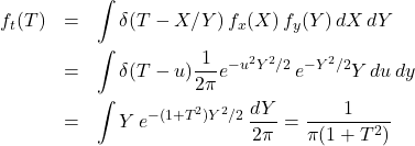
Let ![]() and
and ![]() be independent, normally distributed. Let
be independent, normally distributed. Let ![]()
(1) 
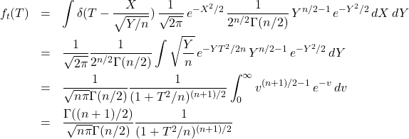
Student’s ![]() -distribution may be a little less obvious. The
-distribution may be a little less obvious. The ![]() -statistic can be written as
-statistic can be written as ![]() in which
in which ![]() is normally distributed being a sum/difference of means, and
is normally distributed being a sum/difference of means, and ![]() has an independent
has an independent ![]() -variable
-variable ![]() distribution
distribution
![]()
so that ![]() is distributed as
is distributed as
(2) 
This is a modified Cauchy distribution.
Functions of random variables
![]()
This is used to obtain the PDF of the function ![]() of a random variable
of a random variable ![]() from the PDF of
from the PDF of ![]() , consider that
, consider that
![]()
however this is also the probability the ![]() will be less than
will be less than ![]() ;
;
![]()
Now just take the derivative using Newton’s law to get the PDF of ![]() (and thus proving Theorem 6.1);
(and thus proving Theorem 6.1);
![]()
This is the basis of the so-called inverse method for computing random deviates with some particular PDF.
Example
Let ![]() be a uniform deviate on the interval
be a uniform deviate on the interval ![]() , meaning that
, meaning that ![]() . This is the type of built-in random number generator computer operating systems have. Find the PDF for a random number
. This is the type of built-in random number generator computer operating systems have. Find the PDF for a random number ![]() .
.
First we get our cumulant
![Rendered by QuickLaTeX.com \[\wp_y(y\le \eta)=\wp_x(x\le \eta^{{1\over n}})=\int_0^{\eta^{{1\over n}}} 1 \cdot d\xi=\eta^{{1\over n}}\]](http://abadonna.physics.wisc.edu/wp-content/ql-cache/quicklatex.com-0be7596de2bfa0e0854caf814bc774a6_l3.png)
and finally
![]()
if ![]() .
.
Example
If ![]() is uniformly distributed over
is uniformly distributed over ![]() , find the probabilty density function of
, find the probabilty density function of ![]() .
.
Let ![]()
![]()
Example
Find the distribution of ![]() , where
, where ![]() is a fixed constant and
is a fixed constant and ![]() is uniformly distributed on
is uniformly distributed on ![]() . This arises in ballistics. if a projectile is launched at speed
. This arises in ballistics. if a projectile is launched at speed ![]() and angle
and angle ![]() from the horizontal, its range is
from the horizontal, its range is ![]() .
.
Use the example of the inverse method, for ![]() ;
;
![]()
but we have ![]() ,
, ![]() , and
, and
![]()
and so
![Rendered by QuickLaTeX.com \[g^{-1}(\eta)={1\over 2} \sin^{-1}\Big({g\eta\over v_0^2}\Big), \qquad {dg^{-1}(\eta)\over d\eta}={1\over 2} {1\over\sqrt{({v_0^2\over g})^2-\eta^2}}\]](http://abadonna.physics.wisc.edu/wp-content/ql-cache/quicklatex.com-ae050d9c1e01a48eada6b1218d16516e_l3.png)
and so the ranges are distributed according to
![Rendered by QuickLaTeX.com \[f_R(\eta)=f_g(\eta)={1\over 2\pi} {1\over\sqrt{({v_0^2\over g})^2-\eta^2}}\]](http://abadonna.physics.wisc.edu/wp-content/ql-cache/quicklatex.com-ff4a3938d06fd054d9374bb9dffbf126_l3.png)
The cumulative probability ![]() will be an inverse sine function (verify).
will be an inverse sine function (verify).
Example (Problem 5.16 in Ross)
In ![]() independent tosses of a coin the coin landed heads
independent tosses of a coin the coin landed heads ![]() times. Is it reasonable to assume that the coin is fair?
times. Is it reasonable to assume that the coin is fair?
What is the probability of landing within one ![]() of
of ![]() the mean for a normal distribution?
the mean for a normal distribution?
![]()
![]()
The probability of landing within two ![]() of
of ![]() the mean is
the mean is
![]()
![]()
For ![]() coin tosses the probability of
coin tosses the probability of ![]() heads will be normally distributed about the mean
heads will be normally distributed about the mean ![]() with
with ![]() . This coin is turning up heads
. This coin is turning up heads ![]() standard deviations beyond the mean, this is not a fair coin.
standard deviations beyond the mean, this is not a fair coin.
Example
If ![]() is uniformly distributed on
is uniformly distributed on ![]() find the pdf of
find the pdf of ![]() .
.
Let ![]()
![]()
![]()