ML/AI: Probability and statistics for ML-1. Basics

These are excerpts from a 300-level course that I taught for a Math department from the excellent book “A First Course in Probability” by Sheldon Ross. Hopefully they will provide you with all that you need for Physics 715 and to understand applications in machine learning.

Consider a sample space $S$ comprised of events or objects, and subsets $E$ and $F$ such that $E\subset S, \, F\subset S$ .

Example
Consider three coin tosses, all independent. What is the sample space $S$ of outcomes?
To solve this you must generate all possible outcomes, by simply dreaming them up from experience,

$S=\{ (hhh),(hht),(hth),(thh),(htt),(tht),(tth),(ttt)\}$

or by using a {\bf cominatorial} counting or generating function

$G(h,t)=\Big(h+t\Big)^3=hhh+hht+hth+thh+htt+tth+tht+ttt$

We define the union of two subsets $E$ and $F$ of $S$ to be the collection of elements of $S$ that are either in $E$ , or in $F$ , or in both $E$ and $F$ , and denote the union as $E\bigcup F$ . The collection of events both in $E$ and $F$ we call the intersection and denote this one of two ways;

$E\bigcap F\equiv EF$

The collection of events in $S$ but not in $E$ we call the complement of $E$ and denote it as $E^c$ .

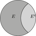
Then we have two extremely useful and important statements

$S=E\bigcup E^c, \qquad F=EF\bigcup E^c F$

both of which you can prove with Venn diagrams. Notice that $EF$ and $E^cF$ are mutually exclusive sets; they have an empty intersection

$EF\bigcap E^cF=\emptyset$

Unions and intersections can be shown via Venn diagrams to satisfy basic properties of algebraic binary operations, such as associativity, commutativity and distribution property

$(E\bigcup F)\bigcup G=E\bigcup(F\bigcup G), \qquad E\bigcup F=F\bigcup E$

$(E\bigcup F)G=EG\bigcup FG$

$EF=FE, \qquad E(FG)=(EF)G$

(it would be a good exercise to draw Venn diagrams illustrating these points).

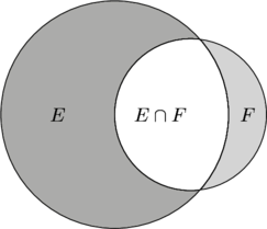
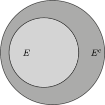
Consider a sample space $S$ and an experiment whose outcome is always some element of $S$ . Repeat the experiment many times under identical conditions. Let $n(e)$ be the number of times in the first $n$ repetitions that the result $e\in S$ we get outcome $e$ . We define the probability of this outcome as

$\wp(e)=\lim_{n\rightarrow\infty} {n(e)\over n}$

Example. Toss three coins, what is the probability of $2$ heads in any order? From the previous page we see $n=8$ and $n(e)=3$ , so $\wp(e)=3/8$ .
Example. The Gibbs microcanonical distribution. All possible states of a system of energy $\epsilon$ , which of course is $S(\epsilon)$ , are equally likely, so the probability that the system is in any one of these states $s$ of energy $\epsilon$ is

$\wp(s)={1\over S(\epsilon)}$

Fundamental properties of probabilities can be derived from the following propositions, all of which are fairly simple to prove:

(1) $\begin{eqnarray*} 1. &\quad & 1=\wp(S)=\wp(E)+\wp(E^c)\nonumber\\ 2. &\quad & E\subset F \Longrightarrow \wp(E)\le \wp(F)\nonumber\\ 3. &\quad & \wp(E\bigcup F)=\wp(E)+\wp(F)-\wp(EF)\nonumber\end{eqnarray*}$

Proof.

$\wp(E\bigcup F)=\wp(E\bigcup E^cF)=\wp(E)+\wp(E^cF)$

this is certainly true since the two sets are mutually exclusive. However $F=EF+E^cF$ and so

$\wp(F)=\wp(EF)+\wp(E^cF)$

again since both of these sets are mutually exclusive. This implies that

$\wp(E^cF)=\wp(F)-\wp(EF)$

and we simply insert this into the first line of the proof, thereby proving 3.

Example An urn contains 3 red, 7 black balls. Players A and B draw balls from the urn consecutively until a red ball is drawn. Find the probability that A selects the red ball. Note that the balls are not replaced in the urn.
The prob of success on the first try for A is $\wp_1={3\over 3+7}={3\over 10}$ , of failure $\wp'_1={7\over 10}$ . Probability of success by B is ${3\over 9}$ and failure is ${6\over 9}$ . Success on the second try for A is contingent upon failure at the first of A followed by failure of B, , $\wp_2=\Big({7\over 10}\Big)\Big({6\over 9}\Big)\Big({3\over 8}\Big)$ since at that stage two of the balls have been removed. Continue, first success at each drawing are mutually exclusive (such probabilities add)

$\wp_A=\wp_1+\wp_2+\cdots={3\over 10}+\Big({7\over 10}\Big)\Big({6\over 9}\Big)\Big({3\over 8}\Big)+\Big({7\over 10}\Big)\Big({6\over 9}\Big)\Big({5\over 8}\Big)\Big({4\over 7}\Big)\Big({3\over 6}\Big)$

$+\Big({7\over 10}\Big)\Big({6\over 9}\Big)\Big({5\over 8}\Big)\Big({4\over 7}\Big)\Big({3\over 6}\Big)\Big({2\over 5}\Big)\Big({3\over 4}\Big)$

Example An urn contains 5 red, 6 blue balls and 8 green balls. If a set of 3 is randomly selected, what is the probability that each will be the same color? Repeat with the assumption that when drawn a balls color is noted and then it is put back into the urn.
Probability that all three drawn are same color;

$\wp=\Big({5\over 19}\Big)\Big({4\over 18}\Big)\Big({3\over 17}\Big)+\Big({6\over 19}\Big)\Big({5\over 18}\Big)\Big({5\over 17}\Big)$

$+\Big({8\over 19}\Big)\Big({7\over 18}\Big)\Big({6\over 17}\Big)$

With replacement;

$\wp=\Big({5\over 19}\Big)^3+\Big({6\over 19}\Big)^3+\Big({8\over 19}\Big)^3$

Example
Urn A contains 3 red and 3 black balls, urn B contains 4 red and 6 black balls. If a ball is selected from each urn, what is the probability that they will be the same color?

$\wp=\Big({3\over 6}\Big)\Big({4\over 10}\Big)+\Big({3\over 6}\Big)\Big({6\over 10}\Big)={1\over 2}$

Example
A town has 4 TV repairmen. If 4 sets break down, what is the probability that exactly $i$ of the repairmen will be called, for $i=1,2,3,4$ .
$4$ repairmen, $4$ service calls, sample space the routing of the service calls, $4^4$ possible routings

$\wp_{all \, same}={4\over 4^4}={1\over 4^3}={1\over 64}$

$\wp_{all \, diff}={4\cdot3\cdot2\cdot 1\over 4^4}={6\over 4^3}={6\over 64}$

Let’s use a generating function (a partition function). Count up sum of coefficients of terms in which only two of the repairman symbols $x,y,z,w$ occur $\wp_{2}={12\cdot 4+6\cdot 6\over 4^4}={21\over 64}$ or terms in which $3$ of the four symbols appear; $\wp_{3}={12\cdot 12\over 4^4}={9\over 16}$ .

$G=(x+y+z+w)^4$

$=\sum_{a,b,c,d}{4!\over a!b!c!d!}x^a y^bz^cw^d, \quad 4^4\cdot \wp(n)=\left\{\begin{array}{ll} 1 & 4{4!\over 4!0!0!0!}\\ 2 & {4\cdot 3\over 2}{4!\over 2!2!0!0!}+4\cdot 3 {4!\over 3!1!0!0!}\\ 3 & 4\cdot 3{4!\over 2!1!1!0!}\\ 4 & {4!\over 1!1!1!1!}\end{array}\right.$

Conditional probability
We define the conditional probability ala’ Kolmogorov that $E$ will occur given that $F$ has already occurred as $\wp(E|F)$ (conditioning on $F$ ). Notice that

$\wp(E|F)\ne \wp(F|E)$

in general. This can also be taken to be an axiom of probability theory.

Example Suppose that on a multiple choice exam in which each question has $m$ possible choices, a student has a probability $p$ of knowing ( $K$ ) the answer to a problem , and a probability of ${1\over m}$ of guessing the correct answer if he or she must guess. Let $\wp(C)$ be the probability that the student gets a problem correct. Let $\wp(K)=p$ be the probability that the student actually knows the correct answer. Then it is clear that

$\wp(C|K)=1, \quad \wp(C|K^c)={1\over m}$

since the student will mark it correct if they know the answer, and must guess if they do not.
The fundamental tools for working with conditional probabilities are
$\bullet$

$\wp(E|F)={\wp(EF)\over \wp(F)}$

which implies

$\wp(EF)=\wp(E|F) \wp(F)=\wp(F|E) \wp(E)$

and
$\bullet$ Bayes’ Theorem

(2) $\begin{eqnarray*} \wp(E)&=&\wp(EF)+\wp(EF^c)\nonumber\\ &=&\wp(E|F)\wp(F)+\wp(E|F^c)\wp(F^c)\nonumber\\ &=&\wp(E|F)\wp(F) +\wp(E|F^c)(1-\wp(F))\nonumber\end{eqnarray*}$

Example Under the conditions of the previous example, what is the probability that a student actually knows the answer if he or she did answer it correctly? This is a standard course-in-probability exam problem.

$\wp(K|C)={\wp(KC)\over\wp(C)}$

$={\wp(C|K)\wp(K)\over \wp(C|K)\wp(K)+\wp(C|K^c)(1-\wp(K))}={mp\over 1+(m-1)p}$

For the record, lets compute a few other quantities;

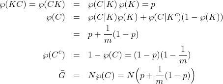
(3) $\begin{eqnarray*}\wp(KC)=\wp(CK)&=&\wp(C|K) \, \wp(K)=p\nonumber\\ \wp(C)&=&\wp(C|K)\wp(K)+\wp(C|K^c)(1-\wp(K))\nonumber\\ &=&p+{1\over m}(1-p)\nonumber\\ \wp(C^c)&=&1-\wp(C)=(1-p)(1-{1\over m})\nonumber\\ \bar{G}&=&N\wp(C)=N\Big(p+{1\over m}(1-p)\Big)\nonumber\end{eqnarray*}$

where the last quantity is the average expected grade on an exam with $N$ multiple choice questions.

We say that two events $E$ and $F$ are independent if

$\wp(EF)=\wp(E)\wp(F)$

Example Consider an experiment in which independent trials, each with a probability of success equal to $p$ , will be performed in success. If $n$ trials are performed, find the probability that there will be at least one success among them.

$\wp(E_1 E_2\cdots E_n)=\prod_i \wp(E_i)$

let each $E_i$ be failure;

$\wp(E_1 E_2\cdots E_n)=(1-p)^n$

and so the probability of at least one success is

$\wp=1-(1-p)^n$

Since each event is independent.

Example Prove that if $\wp(E_i|E_1\cdots E_{i-1})>0$ , for $i=1,2,\cdots,n$ then\\ $\wp(E_1E_2\cdots E_n)=\wp(E_1)\wp(E_2|E_1)\wp(E_3|_1E_2)\cdots \wp(E_n|E_1E_2\cdots E_{n-1})$ .
Start with

$\wp(E_2|E_1)={\wp(E_1E_2)\over \wp(E_1)}, \quad \wp(E_3|E_1E_2)={\wp(E_1E_2E_3)\over \wp(E_1E_2)}$

$\wp(E_4|E_1E_2E_3)={\wp(E_1E_2E_3E_4)\over \wp(E_1E_2E_3)},\cdots$

just multiply all of these together

$\wp(E_1E_2E_3\cdots)=\Big(\wp(E_1)\Big)\Big({\wp(E_1E_2)\over \wp(E_1)}\Big)\Big({\wp(E_1E_2E_3)\over \wp(E_1E_2)}\Big)\Big({\wp(E_1E_2E_3E_4)\over \wp(E_1E_2E_3)}\Big)\cdots$

Example Prove that if $E_1,E_2,\cdots E_n$ are independent events, then $\wp(E_1\cup E_2\cup\cdots\cup E_n)=1-(1-\wp(E_1))(1-\wp(E_2))\cdots (1-\wp(E_n))$ .
This follows from inclusion/exclusion, or from

$\wp(E_1^cE_2^c\cdots E_n^c)=\wp(E_1^c)\wp(E_2^c)\cdots \wp(E_n^c)$

for independent events, with

$\wp(E_1\cup\cdots\cup E_n)=1-\wp(E_1^cE_2^c\cdots E_n^c)$

and $\wp(E_i^c)=1-\wp(E_i)$ .

Example Prove directly that $P(E|F)=P(E|FG) \, P(G|F)+P(E|FG^c) \, P(G^c|F)$ .

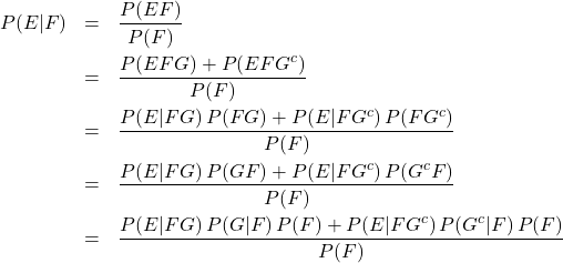
(4) $\begin{eqnarray*} P(E|F)&=&{P(EF)\over P(F)}\nonumber\\ &=&{P(EFG)+P(EFG^c)\over P(F)}\nonumber\\ &=&{P(E|FG) \, P(FG)+P(E|FG^c) \, P(FG^c)\over P(F)}\nonumber\\ &=&{P(E|FG) \, P(GF)+P(E|FG^c) \, P(G^cF)\over P(F)}\nonumber\\ &=&{P(E|FG) \, P(G|F) \, P(F)+P(E|FG^c) \, P(G^c|F) \, P(F)\over P(F)}\nonumber\end{eqnarray*}$

Example Three cards are randomly drawn, without replacement from a deck of 52 playing cards. Find the conditional probability that the first card is a spade, given that the second and third cards are spades.

$\wp(sss)=(13/52)(12/51)(11/50), \quad \wp(ss^cs)=(13/52)(39/51)(12/50)$

$\wp(sss^c)=(13/52)(12/51)(39/50), \quad \wp(s^css)=(39/52)(13/51)(12/50)$

$\wp(first \, s|xss)={\wp(sss)\over \wp(sss)+\wp(s^css)}={13\cdot 12\cdot11\over 13\cdot 12\cdot 11+39\cdot 13\cdot 12}={11\over 50}$

Example Suppose that $5\%$ of men and $0.25\%$ of women are colorblind. A colorblind person is chosen at random from a population containing equal numbers of men and women. What is the probability of it being a man?
$\wp(cb|f)=0.0025$ , $\wp(cb|m)=0.05$ , $\wp(m)=\wp(f)=0.5$ ;

$\wp(m|cb)={\wp(cb|m)\wp(m)\over \wp(cb|m)\wp(m)+\wp(cb|f)\wp(f)}={20\over 21}$

Conditional probabilities in quantum mechanics
Start with $|\psi\rangle$ and consider measurement with $\hat{J}$ , with eigenspace $\{j, \quad |j\rangle\}$ . This is a complete basis of $\mathcal{H}$ so that

$|\psi\rangle=\sum_j \psi_j |j\rangle\quad\mbox{alternatively}\quad \hat{\rho}=\sum_j\wp_j \, |j\rangle\langle j|$

Consider operator $\hat{A}$ , with eigenspace $\{a, \quad |a\rangle\}$ . We can consider

$\wp_{(a|j)}=\langle j|\hat{P}_a|j\rangle=\langle j|a\rangle\langle a|j\rangle=Tr\Big(\hat{P}_a \, |j\rangle \langle j|\Big)$

to be the conditional probability that if the state of the system is one of definite $\hat{J}$ (namely $j$ ) then measurement of $\hat{A}$ results in $a$ . Summing over all conditional probabilities gives the total probability that measurement of $\hat{A}$ results in $a$

$\wp_a=\sum_j \wp_j\wp_{(a|j)}=\sum_j \wp_j \, Tr\Big(\hat{P}_a \, |j\rangle \langle j|\Big)$

$=Tr\Big(\sum_j \wp_j|j\rangle \langle j|\, \hat{P}_a\Big)=Tr\Big(\hat{\rho}\hat{P}_a\Big)$

Baye’s theorem

$\wp_{(j|a)}={\wp_j \wp_{(a|j)}\over \wp_a}$

let’s us construct conditional density matrices; if the system is in state $|j\rangle$ (eigenstate of $\hat{J}$ ) before an $\hat{A}$ measurement is made, after measuring $\hat{A}$ and getting $a$ the system is in state

$|a;j\rangle={\hat{P}_a|j\rangle\over \sqrt{\wp_{(a|j)}}}$

and summing over initial pure states (using Hermiticity of $\hat{P}_a$ and cancellation of some phase factors)

$\hat{\rho}_a=\sum_j \wp_{(j|a)}|a;j\rangle\langle a;j|=\sum_j {\wp_j \wp_{(a|j)}\over \wp_a}|a:j\rangle\langle a;j|$

$=\sum_j {\wp_j \wp_{(a|j)}\over \wp_a}{\hat{P}_a|j\rangle\over \sqrt{\wp_{(a|j)}}}{\langle j|\hat{P}_a\over \sqrt{\wp_{(a|j)}}}=\sum_j {\wp_j \over \wp_a}\hat{P}_a|j\rangle\langle j|\hat{P}_a$

$=\hat{P}_a{\sum_j \wp_j|j\rangle\langle j|\over \wp_a}\hat{P}_a={\hat{P}_a\hat{\rho}\hat{P}_a\over \wp_a}={\hat{P}_a\hat{\rho}\hat{P}_a\over Tr(\hat{P}_a\hat{\rho})}$

Home 2.0

ML/AI: Probability and statistics for ML-1. Basics

Related Posts

ML/AI: Probability and statistics for ML-1. Basics

Published by Jeff on November 27, 2021November 27, 2021

Related Posts

ML/AI: Probability and statistics-III. Continuous random variables

Algorithms: gradient descent

Protected: ML: RandomForest regression in julia